← Notes

Filtering, Estimation, And Kalman Filters

A curated public version of my Obsidian notes while working through Roger Labbe’s Kalman and Bayesian Filters in Python and Thrun, Burgard, and Fox’s Probabilistic Robotics.

Filtering is the problem of estimating hidden state from imperfect information. A sensor reading is not the state. It is evidence about the state. A motion model is not the state either. It is a prediction about how the state should evolve. A useful filter keeps both sources of information and weights them by how trustworthy they are.

That principle is the thread from simple g-h filters to histogram Bayes filters to Kalman filters:

1. Predict what the system should do next.
2. Compare that prediction with a measurement.
3. Move the estimate by an amount justified by uncertainty.
4. Carry the new estimate and uncertainty into the next step.

Independent imperfect measurements can produce a better estimate when their uncertainties are modeled. The fused estimate moves toward the more precise source and becomes narrower than either source alone.

Noisy Sensors

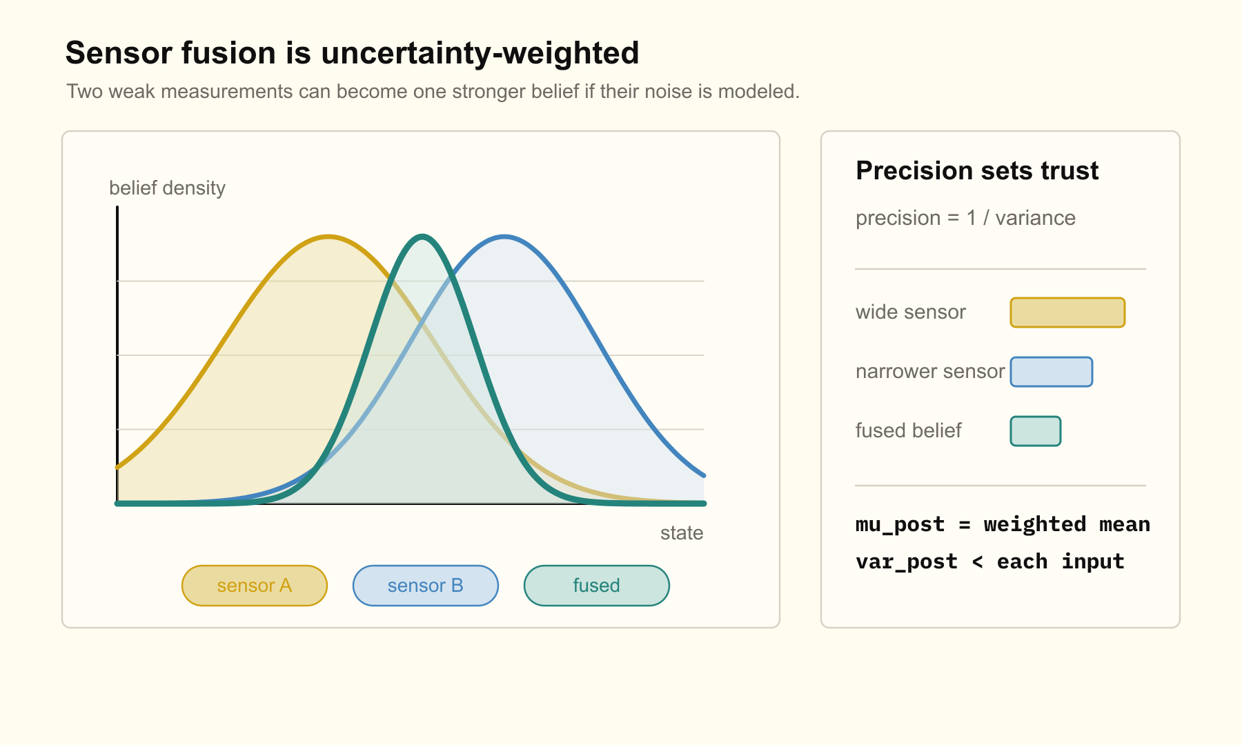
Sensors are inaccurate by design in the sense that they measure the world through noise, bias, resolution limits, latency, calibration drift, and environmental effects. The right response is not to throw away a noisy reading. It is to model how noisy the reading is.

For two independent scalar Gaussian estimates, the cleanest form is precision weighting:

$$\mu =\frac{{\tau }_1{\mu }_1+{\tau }_2{\mu }_2}{{\tau }_1+{\tau }_2},{\tau }_i=\frac{1}{{\sigma }_i^2}$$

Precision is inverse variance. A smaller variance gives a larger precision, so the fused mean moves closer to the more reliable estimate. The fused variance becomes:

$${\sigma }^2=\frac{1}{{\tau }_1+{\tau }_2}$$

This is the mathematical version of the note’s rule: never discard information when the uncertainty model is credible. The estimate should land between the inputs, and the uncertainty should reflect how much evidence supports it.

Predictor-Corrector Loop

A filter becomes useful when measurements arrive over time. At each epoch, it alternates between a prediction step and an update step.

Prediction propagates the state through a process model and increases uncertainty. Measurement update uses the residual to correct the state and usually reduces uncertainty.

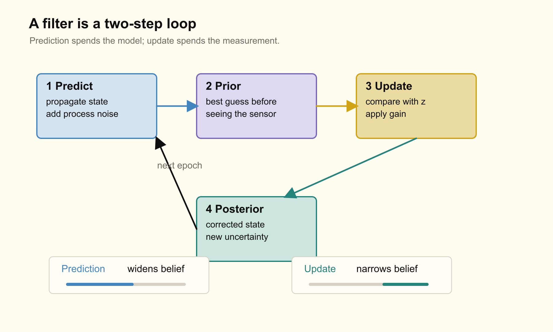
The prediction step uses a process model:

$${\hat{x}}_k^{-}=f({\hat{x}}_{k-1}^{+},u_k)$$

The update step compares the measurement with what the prediction expected:

$$r_k=z_k-h({\hat{x}}_k^{-})$$

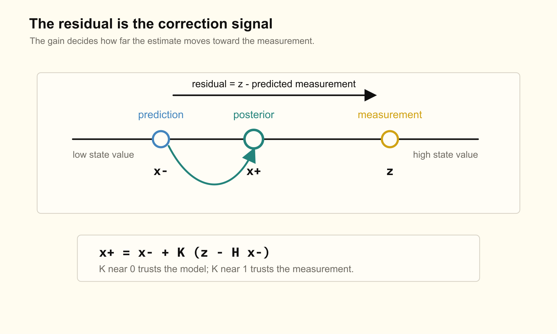
The residual, also called the innovation, is the part of the measurement not explained by the prediction. A scalar update has the form:

$${\hat{x}}_k^{+}={\hat{x}}_k^{-}+K_k{r}_k$$

The gain $K_k$ controls how far the estimate moves toward the measurement. If the prediction is trusted more, $K_k$ is small. If the measurement is trusted more, $K_k$ is large.

The update is a movement along the residual line. The gain determines where the posterior estimate lands between prediction and measurement.

g-h Filters

The g-h filter, also called an alpha-beta filter, is the compact version of this idea for position and rate. It tracks a value $x$ and its rate $\dot{x}$.

x_pred = x + dx * dt
dx_pred = dx
 
residual = z - x_pred
 
x = x_pred + g * residual
dx = dx_pred + h * residual / dt

The $g$ gain decides how much the position estimate follows the measurement. The $h$ gain decides how much the rate estimate changes after seeing the residual. Large gains react quickly but pass more measurement noise through. Small gains reject noise but lag behind real changes.

Gains are not decoration. They encode a belief about sensor noise and process behavior. Bad gains can look good on one data set and fail when the motion changes.

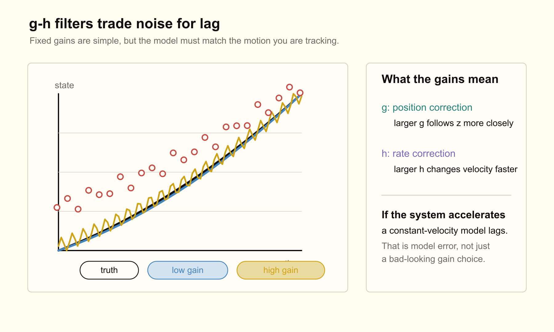
This is why filters are designed, not selected ad hoc. If the real system accelerates but the model assumes constant velocity, no choice of fixed $g$ and $h$ can remove the systematic lag completely. The filter is reporting a modeling mistake, not only a tuning mistake.

Bayesian Filters

Bayesian filtering keeps a belief distribution over state. The prior is the belief before incorporating the new measurement. The posterior is the belief after incorporating it.

For a discrete state space, prediction is:

$$\overline{bel}(x_k)=\sum _{x_{k-1}}p(x_k\mid u_k,x_{k-1})bel(x_{k-1})$$

Update is:

$$bel(x_k)=\eta p(z_k\mid x_k)\overline{bel}(x_k)$$

The likelihood $p(z_k\mid x_k)$ scores how compatible the measurement is with each possible state. It does not need to sum to one over states; the normalizer $\eta$ turns the product back into a probability distribution.

The motion model spreads belief during prediction. The measurement model concentrates belief during update. The posterior becomes the next cycle's input.

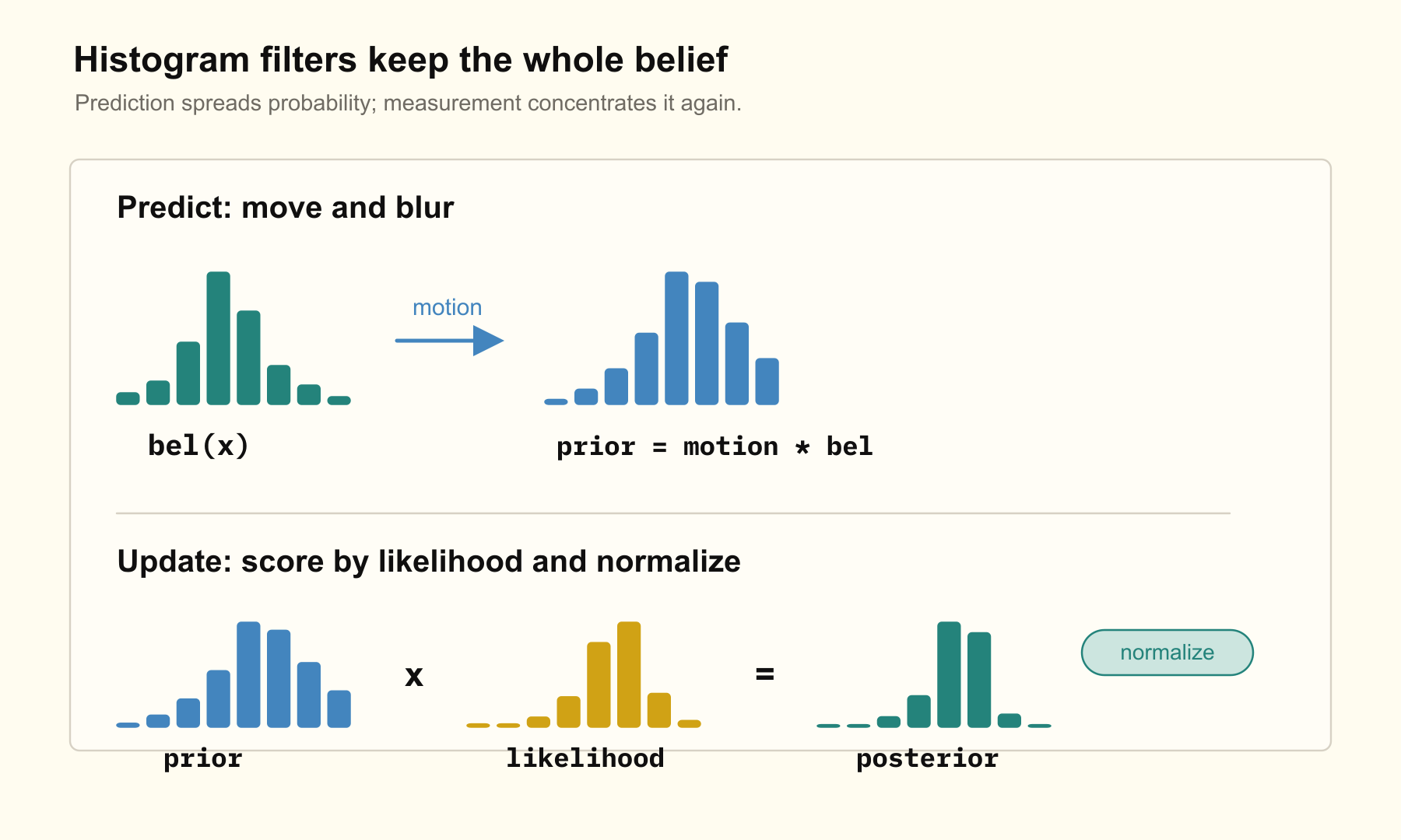
In the hallway example from the notes, the state is a categorical distribution over positions. A motion command shifts the distribution, but uncertainty about the motion spreads probability mass to neighboring cells. For translational motion, this prediction is a convolution between the current belief and a motion-error kernel.

Without probabilities, prediction looks like adding motion to a state estimate. With probabilities, prediction moves and spreads belief. That spreading is information loss. The update step can recover certainty only if the measurement is informative enough.

Histogram filters are powerful because they can represent multimodal belief. They are also expensive because they must update each state cell. In high-dimensional continuous systems, this becomes the pressure that leads to approximations.

The Kalman Bridge

The Kalman filter is the continuous Gaussian version of the same predictor-corrector story. It assumes the belief is summarized by a mean and covariance, and in the basic form it assumes linear dynamics and linear measurements.

Kalman filtering preserves the Bayes filter structure while replacing full distributions with a Gaussian mean and covariance.

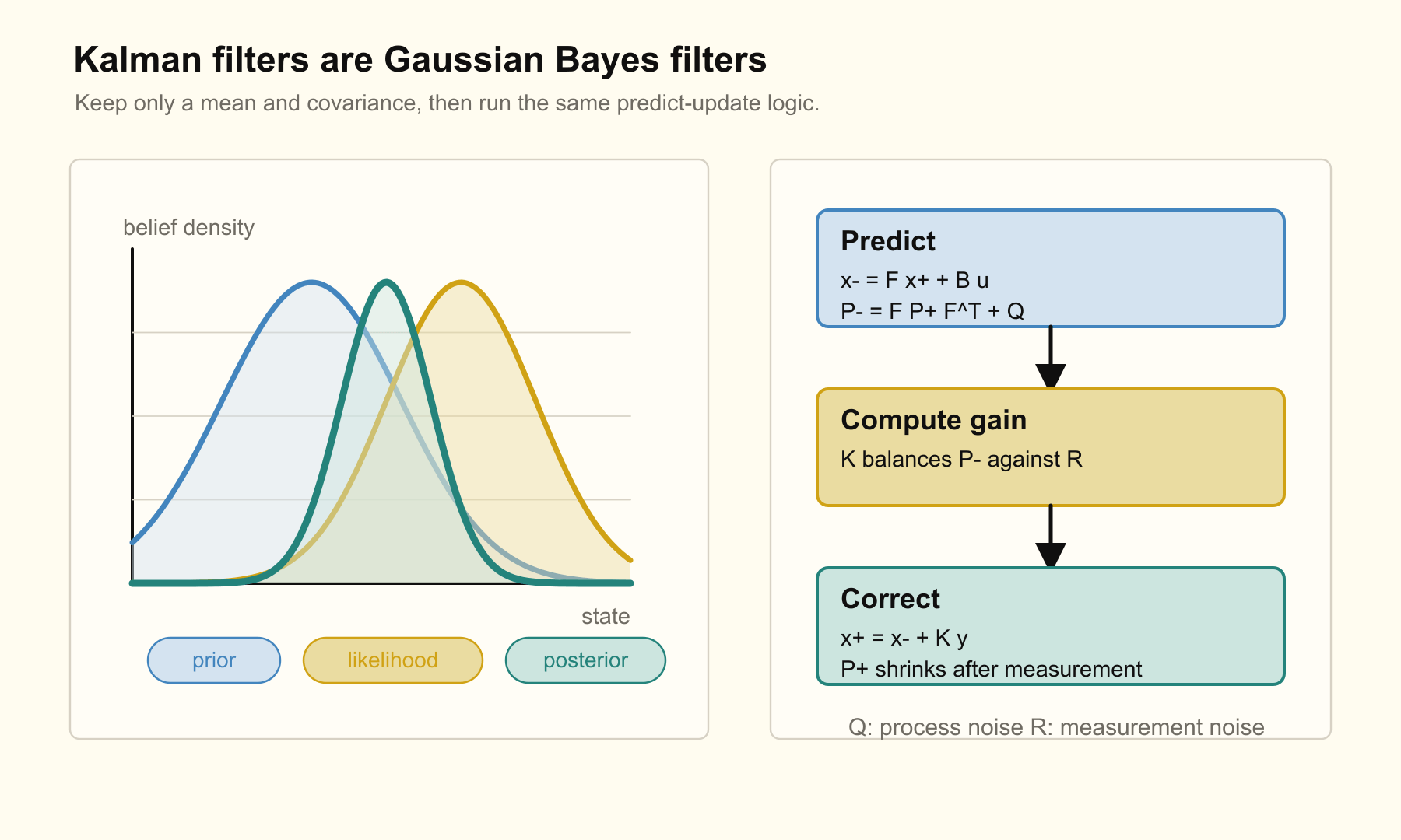
The linear predict step is:

$${\hat{x}}_k^{-}=F_k{\hat{x}}_{k-1}^{+}+B_k{u}_k$$ $$P_k^{-}=F_k{P}_{k-1}^{+}{F}_k^T+Q_k$$

The update step is:

$$y_k=z_k-H_k{\hat{x}}_k^{-}$$ $$K_k=P_k^{-}{H}_k^T(H_k{P}_k^{-}{H}_k^T+R_k{)}^{-1}$$ $${\hat{x}}_k^{+}={\hat{x}}_k^{-}+K_k{y}_k$$

Here $P$ is state uncertainty, $Q$ is process noise, $R$ is measurement noise, and $H$ maps state into measurement space. The Kalman gain is not a magic knob. It is the consequence of the relative uncertainty in the prediction and the measurement.

This is the compact connection: a g-h filter uses fixed gains, a histogram Bayes filter carries an explicit probability table, and a Kalman filter carries a Gaussian belief through linear algebra. All three ask the same question at every step: given my model and my measurement, how much should my belief move?

Open Questions

• How can a filter detect model drift when the changing part of the process is not directly measured?
• When should lag be treated as a tuning problem, and when is it evidence that the state model needs acceleration or a different process term?
• How should gains or covariance terms be chosen from real sensor behavior instead of tuned to one convenient data set?
• Where does the histogram filter become computationally unreasonable, and what approximation should replace it?
• Which tracking problems require preserving multimodality with particles instead of collapsing belief to one Gaussian?

References

• Roger Labbe, Kalman and Bayesian Filters in Python
• Roger Labbe, Kalman and Bayesian Filters in Python PDF
• Sebastian Thrun, Wolfram Burgard, and Dieter Fox, Probabilistic Robotics
• Thrun, Burgard, and Fox, Probabilistic Robotics official site